Kaggle Titanic
Kaggle Titanic
Preface
I appreciate your understanding regarding any potential errors or omissions, as I’m still in the learning process. Feel free to engage in discussions – I’m here to help and discuss any topics you’d like to explore.
Learning is a continuous journey, and open discussions can lead to valuable insights and growth.
This article begins by exploring the most straightforward approach to address the issue.
If you wish to follow along with my code, please visit my GitHub repository using the following link:
Linermao’s GitHub: https://github.com/Linermao/Kaggle-Code
1. Competition Overview
- Original competation link: Titanic - Machine Learning from Disaster
The sinking of the Titanic is one of the most infamous shipwrecks in history.
On April 15, 1912, during her maiden voyage, the widely considered “unsinkable” RMS Titanic sank after colliding with an iceberg. Unfortunately, there weren’t enough lifeboats for everyone onboard, resulting in the death of 1502 out of 2224 passengers and crew.
While there was some element of luck involved in surviving, it seems some groups of people were more likely to survive than others.
In this challenge, we ask you to build a predictive model that answers the question: “what sorts of people were more likely to survive?” using passenger data (ie name, age, gender, socio-economic class, etc).
2. Data
2.1 Download Data
Firstly, you should install ‘Kaggle’. If you’ve already done this, please disregard this step.
pip install kaggle |
Then, you can utilize this code to download data from the Titanic competition.
kaggle competitions download -c titanic |
Alternatively, you can log in to Kaggle to download the data.
- click hear: https://www.kaggle.com/competitions/titanic/data
Careful! There are three .csv files. But the files we only need are train.csv and test.csv .
2.2 Data Extraction
To start, It is imperative to ascertain the available data and its significance.
import pandas as pd |
Data columns (total 12 columns): |
From the Competition, we know:
| Variable | Definition | Key |
|---|---|---|
| Survival | Survival | 0 = No, 1 = Yes |
| Pclass | Ticket class | 1 = 1st, 2 = 2nd, 3 = 3rd |
| Sex | Sex | |
| Age | Age in years | |
| Sibsp | # of siblings / spouses aboard the Titanic | |
| Parch | # of parents / children aboard the Titanic | |
| Ticket | Ticket number | |
| Fare | Passenger fare | |
| Cabin | Cabin number | |
| Embarked | Port of Embarkation | C = Cherbourg, Q = Queenstown, S = Southampton |
2.3 Data Cleaning
2.3.1 Imputing Missing Values
We observe that ‘Age’, ‘Fare’, ‘Cabin’, and ‘Embarked’ contain missing values, with ‘Cabin’ being particularly notable with a loss of nearly 70% of its values.
The missing values in ‘Survived’ arise from the fact that they need to be predicted based on the model we establish for the test set. Therefore, they can be disregarded for now.
Let’s focus on ‘Age’ as a starting point for analysis.
In handling missing values, the most commonly employed method is to replace them with the mean value.
Thus, we can employ the following code to address the ‘Age’ variable :
data_all['Age'].fillna(data_all['Age'].mean(), inplace = True) |
It’s worth mentioning that using the mean to fill in missing values is an extremely rudimentary and hasty approach. Therefore, we will further optimize our missing value imputation method in subsequent steps.
For ‘Fare’, which has only one missing value, we can replace it with the mean value as well.
data_all['Fare'].fillna(data_all['Fare'].mean, inplace = True) |
Regarding ‘Embarked’, we could analyze its distribution pattern as a reference for our next steps.
print(data_all['Embarked'].value_counts()) |
Embarked |
We can visually observe that the majority of values are distributed around ‘S’, indicating that we can utilize ‘S’ to impute the missing values.
Interestingly, you can print the names of the missing individuals and conduct online searches to confirm that they indeed boarded at the ‘Southampton’ port.
print(data_all[data_all[['Embarked']].isnull().any(axis=1)]) |
PassengerId Survived Pclass Name Sex Age SibSp Parch Ticket Fare Cabin Embarked |
Impute the missing values.
data_all['Embarked'].fillna('S',inplace=True) |
Now, let’s shift our focus to ‘Cabin’. Due to the excessive number of missing values, it might be advisable to remove them for now. However, we will certainly revisit this issue and discuss it separately in the future.
data_all.drop('Cabin',axis=1,inplace=True) |
Lastly, after imputing all the missing values, let’s perform a final check.
print(data_all.isnull().any()) |
False |
2.4 Feature Engineering
Firstly, we observe that the ‘Ticket’ column contains a mix of characters and numbers, which could introduce unnecessary complexity for our initial model. This equally applies to the ‘Name’ column as well. Therefore, we can choose to disregard them for now and revisit the topic later.
data_all.drop('Ticket',axis=1,inplace=True) |
Subsequently, we discover that ‘SibSp’ and ‘Parch’ can be combined to create new variables, I will refer to this new variable as “FamilySize,” which represents the sum of a passenger’s siblings and spouse count plus parent and children count and then adding 1 to account for the passenger themselves.
data_all['FamilySize'] = data_all['SibSp'] + data_all['Parch'] + 1 |
Next, we will group the data by ‘Age’ separately. Grouping can assist us in extracting deeper insights from the data.
data_all['Age'] = pd.cut(data_all['Age'], 5) |
Age |
For ‘Fare’, we can apply similar grouping methods. However, there are some additional aspects to consider.
To begin, we can display the value counts for ‘Fare’.
print(data_all['Fare'].describe()) |
count 1309.000000 |
We observe that while the maximum value is quite high, the mean and median values are comparatively smaller. This suggests that a small portion of individuals purchased expensive tickets, prompting the need to classify this subgroup separately.
The presence of a minimum value of 0 indicates that some individuals boarded for free, possibly indicating workers. We will delve into this matter in more detail later.
We can establish our own classification ranges to roughly categorize different fare tiers. The following is an good example of this.
print(data_all['Fare'].describe(percentiles = [0.6,0.9,0.98])) |
count 1309.000000 |
Actually, we can observe that only four individuals purchased the highest tickets.
The joy of the affluent is beyond comprehension.
print(data_all['Fare'][data_all['Fare'] > 300]) |
258 512.3292 |
Hence, we can proceed with our categorization.
bins = [0, 14, 78, 220, 500, 600] |
Fare |
2.5 One Hot Encoding
Up to this point, we have conducted a preliminary “less refined” selection and transformation of the data. However, the obtained values are not yet in integer or floating-point format, so they cannot be directly fed into the model for training. Another transformation is required.
Allow me to provide you with an easy example:
In the ‘Sex’ column, where the values are either ‘male’ or ‘female’, we should convert these to 1 or 0 respectively, making them compatible for modeling purposes.
We can employ the ‘LabelEncoder’ function from the ‘sklearn.preprocessing’ module for this purpose.
from sklearn.preprocessing import LabelEncoder |
Data columns (total 10 columns): |
We can observe that, except for ‘Survived’, all other columns have been converted to integer type.
Then we can proceed to utilize the One-Hot Encoding technique.
Many algorithms assume that there is a logical sequence within a column. However, this is not always expressed by the numerical ratio. Therefore it is needed to one hot encoding the variables afterwards.
Take an example:
We will transform the ‘Sex’ column into two columns, ‘Sex_1’ and ‘Sex_2’. If ‘Sex’ is 1, then ‘Sex_1’ is set to 1 and ‘Sex_2’ is set to 0, and vice versa.
We employ the ‘get_dummies’ function from the ‘pandas’ module for this purpose.
map_features_2 = ['Pclass','Sex','Embarked','FamilySize','Fare','Age'] |
# Column Non-Null Count Dtype |
Next, we can proceed to separate the original dataset into training and testing sets, preparing for the model training.
train_x = encoded_features.iloc[:traindata.shape[0]] |
3. Model
In this phase, we need to choose an appropriate model to fit the data and select the best-performing model.
3.1 Linear Regression
For a binary classification problem, we can start by attempting the simplest linear regression model.
What we need to do is quite straightforward. We just need to invoke the ‘LinearRegression’ from the ‘sklearn’ package.
from sklearn.linear_model import LinearRegression |
3.2 Logistic Regression
Logistic regression is also one of the commonly used methods for binary classification problems.
from sklearn.linear_model import LogisticRegression |
3.3 Random Forest
from sklearn.ensemble import RandomForestClassifier |
3.4 Output Results
Please pay attention to the required output format as specified in the prompt.
Submission File Format:
You should submit a csv file with exactly 418 entries plus a header row. Your submission will show an error if you have extra columns (beyond PassengerId and Survived) or rows.The file should have exactly 2 columns:
- PassengerId (sorted in any order)
- Survived (contains your binary predictions: 1 for survived, 0 for deceased)
predictions_df = pd.DataFrame({'PassengerId': testdata['PassengerId'], 'Survived': test_y}) |
Then you can proceed to submit your base model to Kaggle. By following my code, you might achieve a score similar to the following:
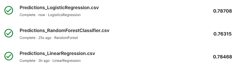
Figure-1 Score
Is it over at this point? No, not by a long shot. What we’ve done so far is just completing a basic model. Let’s not forget that we’ve discarded a significant amount of data and made several simplifications along the way.