Kaggle Titanic Improved
Kaggle Titanic Improved
Preface
Before you begin reading this article, I have a tragic thing to tell you. Despite my belief that the data analysis presented in this article is more systematic and rigorous, the final scores obtained from the data results may not be as ideal. Nevertheless, I still wish to showcase my thought process. After all, the data analysis in the “Base Model” article left much to be desired.
1. Improvements
1.1 Exploratory Data Analysis (EDA)
Firstly, we have a simple idea: could gender be related to survival rate? Because of “Ladies first”.
import seaborn as sns |
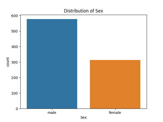
Figure-1 Sex_Numbers
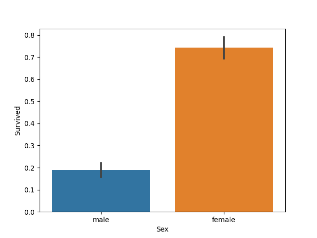
Figure-2 Sex_Survived
We hypothesize that social status could be correlated with survival rate, as depicted in movies where lower-class workers often had fewer opportunities to escape.
plt.hist([data_all[data_all['Survived']==1]['Pclass'],data_all[data_all['Survived']==0]['Pclass']], color = ['g','r'], label = ['Survived','Dead']) |
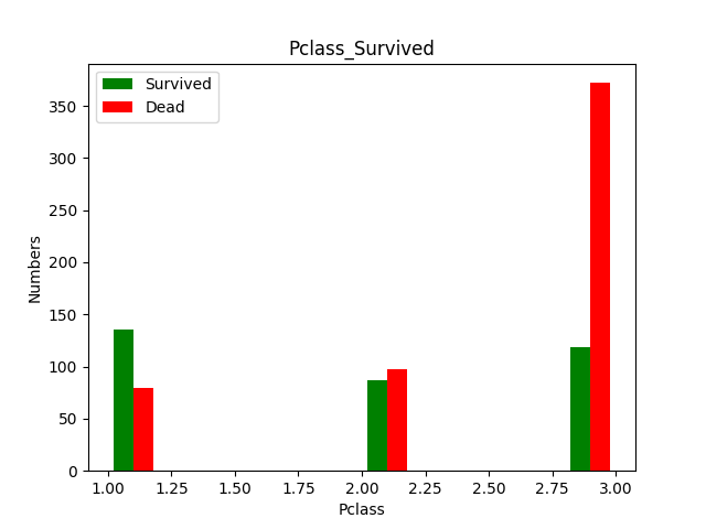
Figure-3 Pclass_Survived
plt.hist([data_all[data_all['Survived']==1]['Fare'],data_all[data_all['Survived']==0]['Fare']],color = ['g','r'], bins = 50, label = ['Survived','Dead']) |
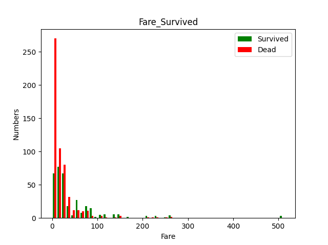
Figure-4 Fare_Survived
Indeed, as it turns out, a higher ticket class is associated with a higher probability of survival.
In other words, higher social status increases the rate of survival.
1.2 Feature Engineering
1.2.1 Cabin
Let’s shift our focus back to the data we previously discarded. We’ll start by analyzing the ‘Cabin’ column.
print(data_all['Cabin'].unique()) |
[nan 'C85' 'C123' 'E46' 'G6' 'C103' 'D56' 'A6' 'C23 C25 C27' 'B78' 'D33' |
We notice that ‘Cabin’ is composed of letters and numbers, with the first letter representing the deck number of the cabin and the second letter denoting the room number. Clearly, the deck number holds more meaningful information for our analysis.
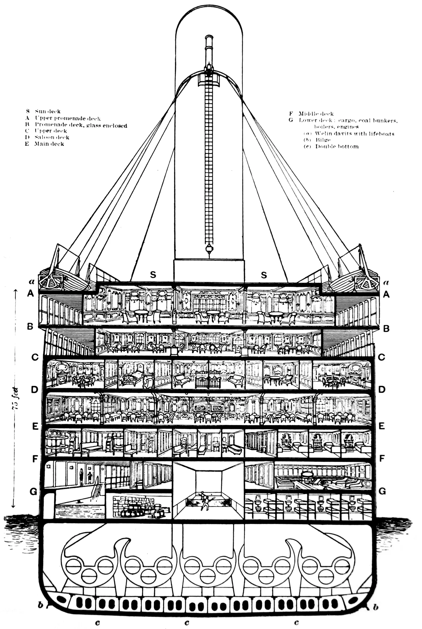
Figure-5 Cabin
Certainly, survival chances were higher for passengers on higher decks. From the chart, we can observe the distribution characteristics of the ‘Cabin’ feature.
Before extracting, I used ‘U’ (unknown) to fill in the missing values as a preliminary step. Then, we will extract the first letter.
data_all['Cabin'].fillna('U',inplace=True) |
Cabin |
Interestingly, there is no information about the ‘T’ cabin here. (Could it be that someone slept on the mast?) Nonetheless, it’s not an issue. Since there is only one ‘T’ cabin data, we can manually assign it to another cabin.
Please note that this is the traindata!
data_all.loc[(data_all['Cabin'] == 'T'), 'Cabin'] = 'F' |
Next, it naturally comes to mind to allocate the ‘U’ data to other categories based on fare levels.
print(data_all.groupby("Cabin")['Fare'].max().sort_values()) |
Cabin |
However, during the grouping process, we discovered that there were passengers in the ‘A’ ‘B’ cabin who boarded for free! They might have been invited as aristocrats.
print(data_all[data_all['Fare'] == 0]) |
PassengerId Survived Pclass Name Sex Age SibSp Parch Ticket Fare Cabin Embarked |
After careful consideration, I’ve decided to assign passengers with ticket class 1 to the ‘B’ cabin.
data_all.loc[(data_all['Fare'] == 0) & (data_all['Pclass'] == 1) &(data_all['Cabin'] == 'U'), 'Cabin'] = 'B' |
Next, we can proceed to group the ‘U’ cabin based on the fare corresponding to each cabin.
def cabin_estimator(i): |
Afterward, I performed another round of subdivision. This can help reduce the number of training parameters and mitigate the potential for overfitting.
data_all['Cabin'] = data_all['Cabin'].replace(['A','B'], 'AB') |
1.2.2 Name
Passenger names are also valuable data. Titles can provide insights into their social status, and first name can indicate whether they have family members onboard. Here, we will extract only the title data.
data_all['Title'] = data_all['Name'].map(lambda name:name.split(',')[1].split('.')[0].strip()) |
['Mr' 'Mrs' 'Miss' 'Master' 'Don' 'Rev' 'Dr' 'Mme' 'Ms' 'Major' 'Lady' |
We can also group the titles. The grouping order is not explained here, and I will provide it directly.
data_all['Title'].replace(['Mlle','Mme','Ms','Dr','Major','Lady','the Countess','Jonkheer','Col','Rev','Capt','Sir','Don','Dona'], |
1.2.3 Age
One’s title can also reflect his age, so we can impute missing values based on the average age associated with each title.
print(data_all.groupby("Title")['Age'].mean().sort_values()) |
Title |
data_all.loc[(data_all['Age'].isnull())&(data_all['Title']=='Mr'),'Age']=33 |
With these processing steps completed, the data has been effectively restored, and we are ready to proceed to the next testing phase.
1.3 Ohters
The rest of the processing methods and the final model code are the same as in the previous article. I’ll come back to fill in the gaps once my skills become more advanced.