NeRF Paper read

1. Preface

This article will introduce NeRF and explain some interesting points from the paper: “NeRF: Representing Scenes as Neural Radiance Fields for View Synthesis” Hereinafter referred to NeRF Paper.

2. What is NeRF

NeRF (Neural Radiance Fields) was first introduced in the best paper presented at ECCV 2020,

We present a method that achieves state-of-the-art results for synthesizing novel views of complex scenes by optimizing an underlying continuous volumetric scene function using a sparse set of input views. Our algorithm represents a scene using a fully-connected (nonconvolutional) deep network, whose input is a single continuous 5D coordinate (spatial location (x, y, z) and viewing direction (θ, φ)) and whose output is the volume density and view-dependent emitted radiance at that spatial location. We synthesize views by querying 5D coordinates along camera rays and use classic volume rendering techniques to project the output colors and densities into an image. Because volume rendering is naturally differentiable, the only input required to optimize our representation is a set of images with known camera poses. We describe how to effectively optimize neural radiance fields to render photorealistic novel views of scenes with complicated geometry and appearance, and demonstrate results that outperform prior work on neural rendering and view synthesis. View synthesis results are best viewed as videos, so we urge readers to view our supplementary video for convincing comparisons.

The above content comes from NeRF Paper.

In short, NeRF is a way to represent complex 3D scenes using only 2D posed images as supervision.

We can refer to the image below, where the input is a lot of 2D photos, and we get a 3D object by using NeRF.

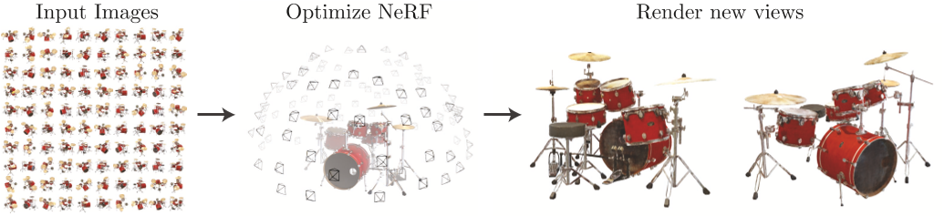
Figure 1.1

(From NeRF Paper)

3. How it works

I use four steps to interpret NeRF:

• Radiance Fields
• Neural Radiance Fields
• Volume Rendering
• Implementation details

Roughly the overall flow is shown in Figure 3.1.

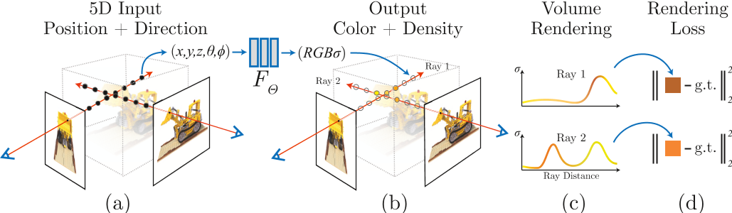
Figure 3.1

(From NeRF Paper)

Let’s interpret it.

3.1 Radiance Fields

All we need to know about Radiance Fields is that it’s a five-dimensional function:

$$\tag{3.1.1} L:X^3 \times W^2 \rightarrow C^3$$ $$\tag{3.1.2} L(x,y,z,\theta,\phi) = (r,g,b)$$

x,y,z represent the coordinates of a certain point in 3D space, and $\theta$, $\phi$ represent the viewing angles in spherical coordinates.

Simply, we can think of radiance field as describing a point in space as an RGB color point.

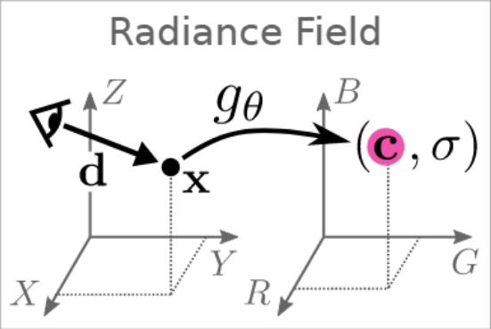
Figure 3.1.1

(From GRAF Paper)

3.2 Neural Radiance Fields

The difference between Neural Radiance Fields and Radiance Fields is that we use MLP to express the function implicitly, and produces another data volume density in addition to RGB data.

$$\tag{3.2.1} L(x,y,z,\theta,\phi) = (r,g,b,\sigma)$$

This is very interesting, it’s like we assume the answer is X, and then we keep revising X to get closer to the correct answer, and obviously we don’t know how to do that, but it does, so the whole process is like a black box model.

In order to optimize our MLP network, we need a way to compare the output with the input, Volume rendering is a good way to do this.

3.3 Volume Rendering

In simple terms, volume rendering is the process of rendering a generated 3D model into a 2D image.

Why would we do this? Because computer screens are 2D! It just looks like it’s 3D.

Maybe this is a little confusing, so let me explain it a little bit more.

When 3D games appeared on the screen, people thought it was incredible. How did this happen? We can assume that the player’s point of view is a laser emitter, we can easily calculate the distance from the laser to the object we encounter in the 2D view, the computer calculates this distance, and renders the illuminated object according to a certain proportion, thus producing a 3D visual effect.

(There was supposed to be a very nice picture here, but I couldn’t find it TOT)

So, once we compressed it back to 2D, we can see the model we generated on the screen.
Let’s assume that a light is emitted from a camera (In computer graphics, light is emitted from a camera). Taking into account all the points on this ray generated by the neural radiance field in the first step, we can use the magic function (3.3.1) to obtain the RGB data of the given point on this ray at this angle.

The magic function is below:

$$\tag{3.3.1} C(\mathbf{r}) = \int_{t_n}^{t_f} T(t) \sigma(\mathbf{r}(t))\mathbf{c}(\mathbf{r}(t),\mathbf{d}) dt,\ where \ T(t) = exp(- \int_{t_n}^{t} \sigma (\mathbf{r}(s))ds)$$

For practical use, we use the discretized formulation:

$$\tag{3.3.2} \hat{C}(\mathbf{r}) = \sum_{i=1}^{N}T_i (1-exp(-\sigma_{i} \delta_{i}))\mathbf{c}_i,\ where \ T(t) = exp(- \sum_{j=1}^{i-1} \sigma_{j} \delta_{j})$$

Where $C$ represents the color, $\sigma$ represents the volume density, $r$ and $d$ represent the distance and direction on the camera ray, and $t$ represents the distance of the sampling point on the camera ray from the camera optical center.

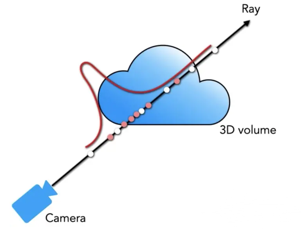
Figure 3.3.1

(From Internet)

Of course, we don’t need to think about how the formula is derived. It takes a little bit of work to figure out this formula, so we’ll come back to it much later.

Since this formulation is naturally differentiable, we can use gradient descent to optimize the network .After a certain number of iterations, we can obtain a perfect network model, which can generate a 3D model from a 2D image.

3.4 Implementation details

In order to improve the accuracy, the position encoding method is also used in the paper.

More details are discussed in the code analysis section.